Introduction
This is one of the coolest looking cellular automata I know of! I found out about it in late 2016 by reading Designing Beauty: The Art of Cellular Automata. The chapter that caught my attention was by David Griffeath but these specific rules were studied with Kellie Evans.
This is a generalization of the Conway's Game of Life which runs on much larger grids. My early implementations failed miserably (ran far too slow to play with) and I let it go for a while. Only when I learned how to write shaders later in October or November of 2017 did I come back and the results were wonderful!
Rules

Cellular automata (CA) are little programs that typically run in a grid of cells. To simplify, each cell has a binary state (0,1) and, at each step of the program, it looks at its neighbor cells' state and decides which state it will have on the next iteration. The Game of Life is a specific set of rules that interprets 0 as being dead, 1 as being alive, uses both orthogonal and diagonal neighbors (of which there are 8) and its rules are:
- A live cell survives if it has 2 or 3 neighbors alive;
- A dead cell is born (becomes alive) if it has 3 neighbors alive;
- All other cells remain as they are (dead or alive).
Larger-than-Life CA, as the name indicates, are similar, but bigger - much bigger. Now you have an additional parameter for the neighborhood-radius (r) which extends neighbors to cells that are at distance at such a distance. In Game of Life, this parameter would always be 1. The number of neighbors, then, is (r+1)*(r+1)-1. The baseline for my images is r=20, which means 440 neighbors. Plus, most GoL simulations have 10 000 - 40 000 cells, whereas here there are more than 1 000 000. All this simply to say that the naive implementation of a CA doesn't really work, especially if you want to maintain interactivity. Fortunately, this kind of parallel computation is what shaders are made for!
Rulers just slightly different, taking upper and lower limits for birth and survival limits. The numbers below are given just as examples since you have a lot more space to maneuver with these large neighborhoods.
- A live cell survives if it has >= 452 and <=1021 neighbors alive;
- A dead cell is born (becomes alive) if it has >= 270 and <=368 neighbors alive;
- All other cells remain as they are (dead or alive).
Coloring
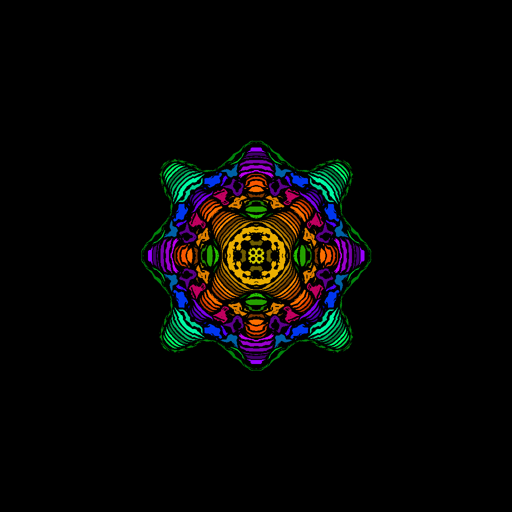
The patterns I've focused on were stable, which means that the pattern grows out of an initial seed and quickly stabilizes into a static image (every live cell survives, no dead cell is born). Coloring these patterns is a simple matter of storing the timestep at which a cell stabilized its state. By applying a modular operation you can get a grayscale image, onto which you can then apply a linear gradient.
The last trick is to apply a luminosity cycling (with an HSL coloring system). Basically, you change the gradient to have a variable luminosity value. Since the patterns have "bands of color", you get a slight variation for each band, which can create some visual interest.


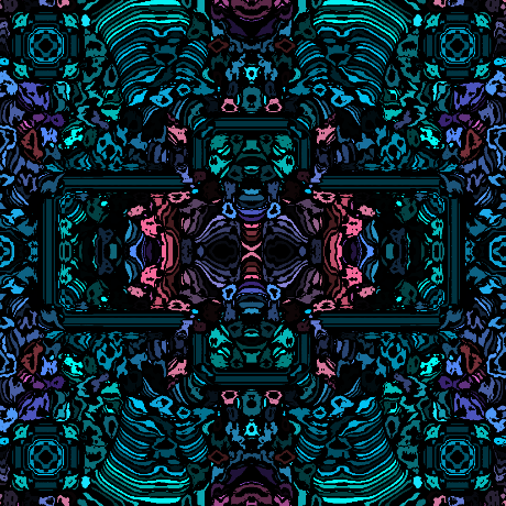
Majority Rule
One cool class of patterns is given by specific set of rules that mimics "conformity". Imagine each cell is a voter that goes with the majority. It looks at its neighbors' states and chooses whichever is most common. Most of the time, the pattern will quickly converge to all 0 or all 1 - however, they take some time to coordinate. This time is stored for coloring, as you know, and you can see the results below. Starting from a random initial state for every cell, you can create many different patterns like the ones below.


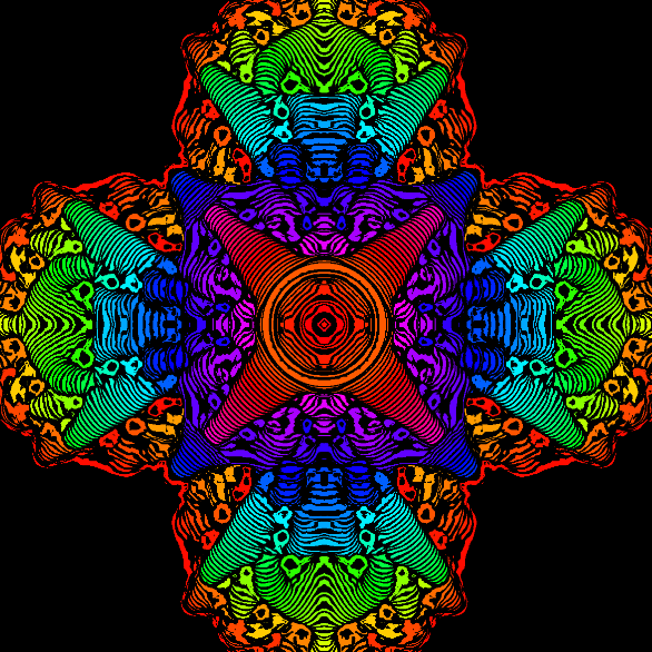
Gallery
Not much else to say about this one. It's beautiful, though, so here are a few more examples!
The first example is a cool one, though it may look no different from the others - but it is a stable pattern. Meaning, while most of the others I've shown will grow until they reach the edge of the screen, this one didn't grow any more.
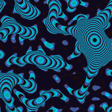
The last example is particularly interesting, and an avenue I did not explore much - that of introducing "obstacles". This breaks up the symmetry (unless you play them symmetrically), with the pattern growing organically around it.